Jet Reports
Conditional Hiding of Rows in Jet Reports
In this tutorial, we will show you how to use conditional hiding of rows in Excel. This useful feature allows you to hide entire rows based on certain criteria. For example, you may want to hide rows where the balance is less than or equal to zero. By using conditional hiding, you can make your reports more concise and easier to read.
We have created a simple report showing the following
Customer No
Customer Name
Balance
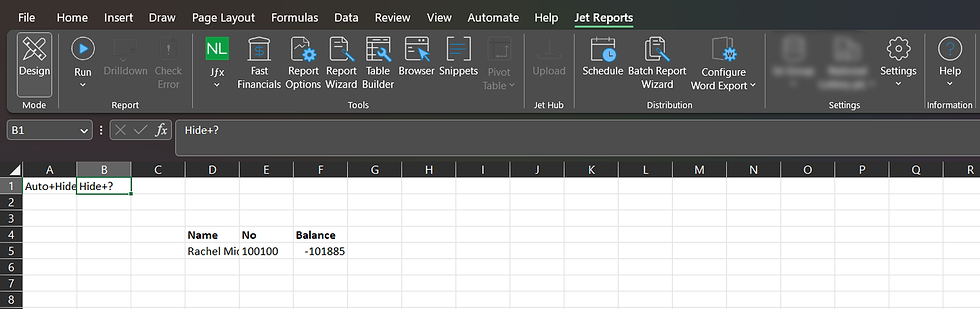
Here is a view of what our report looks like before we apply the conditional hiding

We would like to apply conditional hiding to hide rows where the balance equals zero.
Step 1: Create a Label in Cell B1
To get started, create a label in cell B1. This label should read "Hide+?" and will be used to identify the rows that you want to hide.

Step 2: Use a Formula to Hide Rows Based on Criteria
Next, use a formula to return "Hide" in a row you want to hide. For example, if you want to hide any rows where the balance in cell F5 is less than or equal to zero, you can use the formula "=IF(F5<=0,"Hide","")".

Step 4: Run the Report
After applying the formula and hiding the appropriate rows, run the report to see the changes. Your report should now display only the rows meeting the specified criteria.

In conclusion, conditional hiding of rows is a useful feature that can help you make your reports more concise and easier to read. By following the steps outlined in this tutorial, you can easily use conditional hiding to hide rows based on certain criteria in a professional and friendly manner.